download R Packages For Rs

Text Analysis has been seen as one of the blackboxes of Data Analytics. The aim of this post is to introduce this simple-to-use but effective R package udpipe for Text Analysis.

About udpipe Package

UDPipe — R package provides language-agnostic tokenization, tagging, lemmatization and dependency parsing of raw text, which is an essential part in natural language processing.

Input Dataset

This includes the entire corpus of articles p u blished by the ABC website in the given time range. With a volume of 200 articles per day and a good focus on international news, we can be fairly certain that every event of significance has been captured here. This dataset can be downloaded from Kaggle Datasets.

Summary

Loading required packages for basic Summary :

          library(dplyr)
library(ggplot2)        

Understanding the basic distribution of News articles published:

          news <- read.csv('abcnews-date-text.csv', header = T, stringsAsFactors = F)          news %>% group_by(publish_date) %>% count() %>% arrange(desc(n))          ## # A tibble: 5,422 x 2
## # Groups: publish_date [5,422]
##    publish_date     n
##           <int> <int>
##  1     20120824   384
##  2     20130412   384
##  3     20110222   380
##  4     20130514   380
##  5     20120814   379
##  6     20121017   379
##  7     20130416   379
##  8     20120801   377
##  9     20121023   377
## 10     20130328   377
## # ... with 5,412 more rows        

Plotting to understand how the frequency of headlines is:

          news %>% group_by(publish_date) %>% count() %>% ggplot() + geom_line(aes(publish_date,n, group = 1))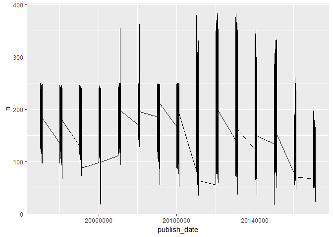        

Before we move on to perform text analysis let's split year, month and date

          library(stringr)          news_more <- news %>% mutate(year = str_sub(publish_date,1,4),
            month = str_sub(publish_date,5,6),
            date = str_sub(publish_date,7,8))        

Let us see the distribution of data based on year:

          news_more %>% group_by(year) %>% count()  %>% ggplot() + geom_bar(aes(year,n), stat ='identity')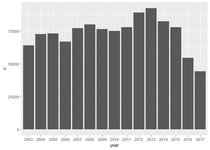        

Pre-trained Model

Udpipe Package provides pretrained language models for respective languages (not programming — but spoken) and we can download the required model using udpipe_download_model()

Loading R package and Getting Language Model ready

          library(udpipe)          #model <- udpipe_download_model(language = "english")
udmodel_english <- udpipe_load_model(file = 'english-ud-2.0-170801.udpipe')        

Filtering data only for 2008

          news_more_2008 <- news_more %>% filter(year == 2008 & month == 10)        

Annotate Input Text Data for 2008

This is the very first function that we'd use in udpipe to get started with our Text Analysis journey. udpipe_annotate() takes the language model and annoates the given text data

          s <- udpipe_annotate(udmodel_english, news_more_2008$headline_text)          x <- data.frame(s)        

Universal POS

Plotting Part-of-speech tags from the given text

          library(lattice)
stats <- txt_freq(x$upos)
stats$key <- factor(stats$key, levels = rev(stats$key))
barchart(key ~ freq, data = stats, col = "yellow",            
            main = "UPOS (Universal Parts of Speech)\n frequency of occurrence",            
            xlab = "Freq")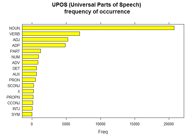        

Most Occurring Nouns

Since we've got the text annotated with Part of Speech, let's understand the most common words of nouns.

          ## NOUNS
stats <- subset(x, upos %in% c("NOUN"))            
stats <- txt_freq(stats$token)
stats$key <- factor(stats$key, levels = rev(stats$key))
barchart(key ~ freq, data = head(stats, 20), col = "cadetblue",            
            main = "Most occurring nouns", xlab = "Freq")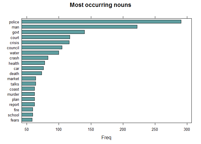        

Ironically, none of the top Nouns that appeared on the newspaper headline just in one month — 10th of 2008, don't bring optimism.

Most Occurring Adjectives

It'd be very hard to find a news agency that doesn't like exaggerating and in English, you exaggerate your object with Adjective. So, let's explore the most occurring Adjectives

          ## ADJECTIVES
stats <- subset(x, upos %in% c("ADJ"))            
stats <- txt_freq(stats$token)
stats$key <- factor(stats$key, levels = rev(stats$key))
barchart(key ~ freq, data = head(stats, 20), col = "purple",            
            main = "Most occurring adjectives", xlab = "Freq")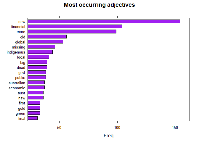        

Most Occurring Verbs

The reporting nature of Media outlets could be very well understood with the way kind of verbs they are using. Do the bring any sign of optimision or they just infuse pessimism? The usage of verbs can answer them.

          ## NOUNS
stats <- subset(x, upos %in% c("VERB"))            
stats <- txt_freq(stats$token)
stats$key <- factor(stats$key, levels = rev(stats$key))
barchart(key ~ freq, data = head(stats, 20), col = "gold",            
            main = "Most occurring Verbs", xlab = "Freq")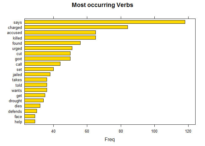        

With words like charged, killed, drought and much more, it doesn't look like the Australian Media outlet wasn't much interested in building an optimistic mindset among its citizens rather like any typical news organization would look for hot, burning, sensational news, it has done the same.

Automated Keywords Extraction with RAKE

Time for some Machine Learning, or let's say simply Algorithms. RAKE is one of the most popular (unsupervised) algorithms for extracting keywords in Information retrieval. RAKE short for Rapid Automatic Keyword Extraction algorithm, is a domain independent keyword extraction algorithm which tries to determine key phrases in a body of text by analyzing the frequency of word appearance and its co-occurrence with other words in the text.

          ## Using RAKE
stats <- keywords_rake(x = x, term = "lemma", group = "doc_id",            
            relevant = x$upos %in% c("NOUN", "ADJ"))
stats$key <- factor(stats$keyword, levels = rev(stats$keyword))
barchart(key ~ rake, data = head(subset(stats, freq > 3), 20), col = "red",            
            main = "Keywords identified by RAKE",            
            xlab = "Rake")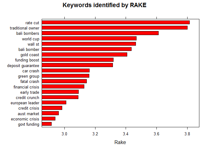        

TOP NOUN — VERB Pairs as Keyword pairs

In English (or probably in many languages), Simple a noun and a verb can form a phrase. Like, Dog barked — with the noun Dog and Barked, we can understand the context of the sentence. Reverse-engineering the same with this headlines data, let us bring out top phrases - that are just keywords/topics

          ## Using a sequence of POS tags (noun phrases / verb phrases)
x$phrase_tag <- as_phrasemachine(x$upos, type = "upos")
stats <- keywords_phrases(x = x$phrase_tag, term = tolower(x$token),            
            pattern = "(A|N)*N(P+D*(A|N)*N)*",            
            is_regex = TRUE, detailed = FALSE)
stats <- subset(stats, ngram > 1 & freq > 3)
stats$key <- factor(stats$keyword, levels = rev(stats$keyword))
barchart(key ~ freq, data = head(stats, 20), col = "magenta",            
            main = "Keywords - simple noun phrases", xlab = "Frequency")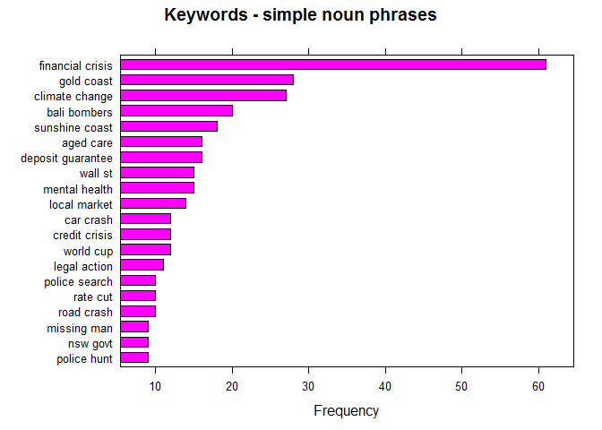        

That concludes the very well-known fact that the 2008 financial crisis was not just a US market meltdown but it was a hot topic all over the world with Australian market not being an exception, this anaylsis lists Financial Crisis at the top along with Wall st after a few topics.

It's also worth noting that this magazine (even though we've seen above that is more interested in highlighting negative news) has helped in making awareness of Climate Change which even the current US President dislikes.

Hope this post helped you get started with Text Analysis in R and if you'd like to know more on Tidy Text Analysis check out this tutorial by Julia Silge. The code used here is available on my github.

Source: https://towardsdatascience.com/easy-text-analysis-on-abc-news-headlines-b434e6e3b5b8

Posted by: hildredboveeer.blogspot.com